Rock, Paper, Scissors (RPS) is a simple classic game. How many plays (or moves) do you have to make (on average) before a game has a winner? Maybe you’d win or lose on the first try, or the second try, but the game surely cannot go that long, right? Let’s find out!

TL; DR

• I made expected value calculations to see how many games one has to play before a game of Rock, Paper, Scissors has a winner
• I compared calulations to simulations
• Repeat, for a few variations of the rule

Instant win

Theory

Let’s explore this problem using both theory and simulations. First, in terms of mathematics, we have 2 in 3 chances of either winning or losing, i.e., the game ends, and 1 in 3 chances of getting a tie. Let \(E[X]\) be the expected number of games taken place, we have:

Let’s break it down! When we play a game of RPS, in 2 in 3 chances, the game ends, the number of game stays the same, but in 1 in 3 chances, the players tie and the number of games increases by 1 (i.e., the game we played), hence \(\frac{1}{3}(E[X] + 1)\). Solving this equation gives us:

Simulations

Let’s compare with simulations!

def rps_result(c1, c2):
    if c1 == c2: return 0
    elif beat[c1] == c2: return 1
    else: return -1

def fast_rps():
    ais = random.choices(['rock', 'paper', 'scissor'], k=2)
    return rps_result(*ais)

# results look to be uniformly distributed
scores = []
for _ in range(10000):
    scores.append(fast_rps())

[(score, scores.count(score)) for score in set(scores)]

[(0, 3313), (1, 3379), (-1, 3308)]

Let’s simulate 1M games of RPS, with each game not stopping until a player wins.

games = []
for _ in range(1000000):
    c, score = 0, 0
    while score == 0:
        score = fast_rps()
        c += 1
    games.append(c)

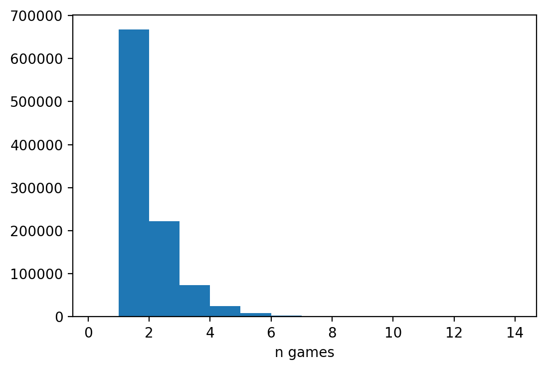
Let’s look at the distribution of the number of games!

def plot_hist(games: list):
    plt.hist(games, bins=range(max(games)))
    
    plt.xlim(-0.5, )
    plt.xlabel('n games')
    
plot_hist(games)
max(games), min(games)

(15, 1)

There are many games of 1, but a game can take up to 8, at least in this simulation. To calculate the expected number of games, we can use the good old:

but in Python, we can use np.mean to simplify it instead.

# close enough
np.mean(games)

1.499318

Two consecutive wins

Great! But what if … we are not content with ending the game after only 1 game? Surely, it does not seem fair to call it win or loss after 1 game. So say, we modify the rule a bit: it now takes 2 consecutive wins (or losses) for the game to have a winner (i.e., if you get a tie in between 2 wins, it does not count). For example, win-win is valid, but win-tie-win would need another win to end the game. How many games (on average) do you have to play now?

Theory

In a way, how this game starts is similar to the other game above: we have 2 in 3 chances a player has a lead, and 1 in 3 chances to get a tie, meaning that the game resets (and the number of games increments by 1). Let \(L\) be the event that a player has a lead, and \(E[X \vert L]\), therefore, be the number of games played when a player has a lead. Intuitively, \(E[X \vert L]\) must be smaller than \(E[X]\) because having a lead means that there would be fewer games to be played compared to when we first started the match. Let’s build the equation:

Let’s break it down! In 1 in 3 chances, the players tie, number of games increases by 1 but we do not get closer to winning or losing. In 2 in 3 chances, however, the number of games now depends on the number of games when someone has a lead. This explanation can be confusing, so an easier way to think about this equation is simplifying the game into its states. There are 3 states of the game:

1. When no one wins or loses, and there is no lead,
2. When someone has a lead, or
3. When someone wins twice (i.e., the game ends).

We start at state (1), and have 2 in 3 chances to reach state (2), and 1 in 3 chances to stay at state (1). The second equation may elucidate this analogy more:

When someone has a lead, there are now 3 scenarios that can follow: someone win another time and the game ends (i.e., state (2) to state (3)), we get a tie and the game goes back to state (1), or the other player wins, which means they now have a lead (i.e., state (2) remains at state (2)). Every time we go to a state where the game continues, the number of games increments by 1. To solve these equations, we can express \(E[X \vert L]\) in terms of \(E[X]\) in the second equation, and substitute it in the first, … or we can use Wolfram Alpha:

Also, as expected, \(E[X \vert H] = \frac{9}{2} \text{ or } 4.5\) which is smaller than 6. On average you should expect to play 6 games of RPS to get a winner. Let’s compare with simulations.

Simulations

games = []
for _ in range(100000):
    c, scores = 0, [0, 0]
    while scores[0] != scores[1] or not any(scores):
        # using a queue
        scores.pop(0)
        scores.append(fast_rps())
        c += 1
    games.append(c)

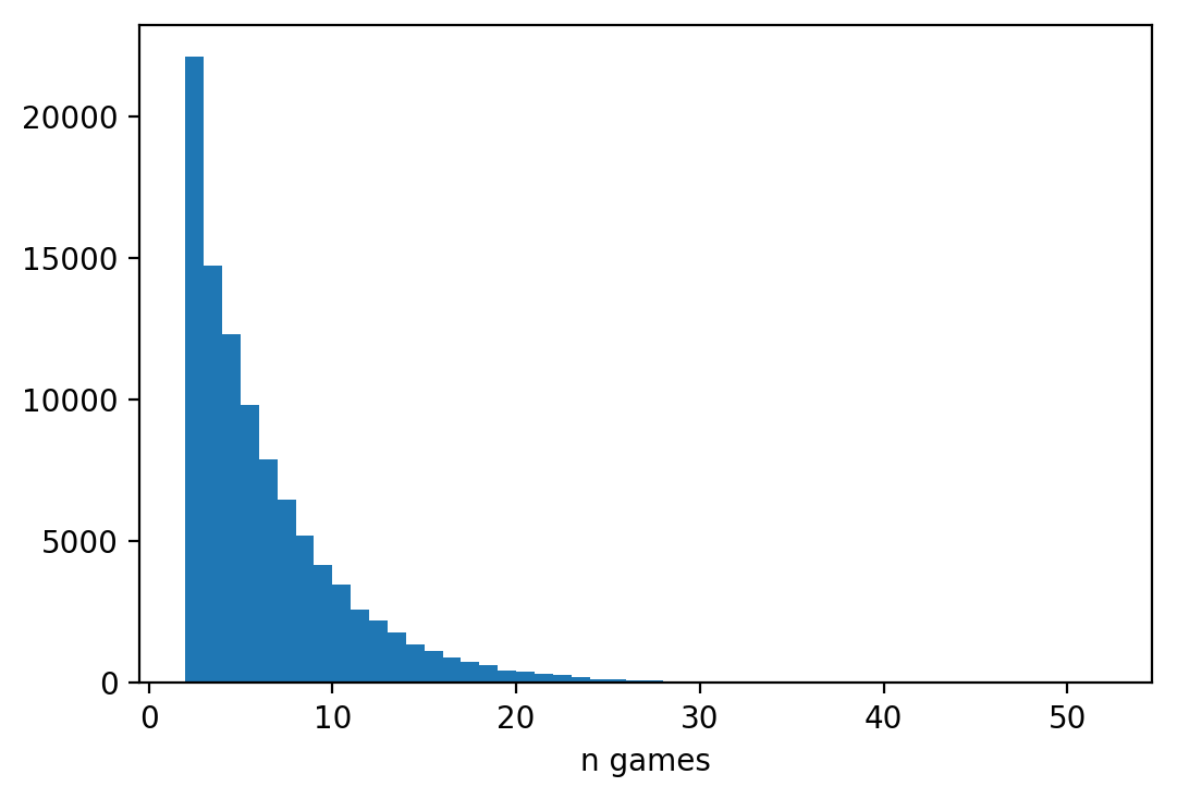
Let’s look at the distribution of the number of games!

plot_hist(games)
max(games), min(games)

(53, 2)

This plot makes sense! There are no game of 1 (of course), and it mostly take 2 to 8 games or up to almost 60 games in total to get a winner!

# close enough?
np.mean(games)

6.02222

Two wins, but not necessarily consecutive

Okay, maybe 6 games (or sometimes, ~60 games) are quite too many to get a winner, so let’s relax the rule a bit: what if ties between 2 wins or losses are acceptable? You need to still win twice, but not consecutively. For example, win-win, win-tie-win, and win-tie-tie-tie-win are all valid wins. How many games should we expect to play until there is an winner?

Theory

Let’s look at the set of equations above:

The first equation should be the same because the new rule does not change how someone can get a lead, but the second equation needs to be modified. The \(\frac{1}{3}(E[X] + 1)\) in the second equation needs to change, because getting a tie now does not move the game state (2) back to (1) (i.e., from someone has a lead to no one has a lead), but holds the game state (2) at (2), with the number of games increasing by 1. Therefore the new equation should be:

Same as above, we can solve for \(E[X \vert L]\) and substitute it to the first equation (or use Wolfram Alpha), which gives us:

Simulations

Let’s compare with simulations!

games = []
for _ in range(100000):

    c, scores = 0, [0, 0]
    while scores[0] != scores[1] or not any(scores):
        s = fast_rps()
        # only wins and losses are added to the queue
        if s != 0:
            scores.pop(0)
            scores.append(s)
        c += 1
    games.append(c)

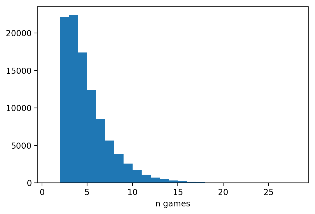
plot_hist(games)
max(games), min(games)

(29, 2)

Interesting! The upper bound of number of games really decreases drastically, despite the number of games expected differs only by 1.5 games.

# close enough!
np.mean(games)

4.49007

OK, cool, so what?

Well, I can tell you about how this experiment is neat because people can expect game time based on expected value or whatever. There is even a tournament in RPS, and if you can imagine how long the entire tournament would take depending on the rule of winning the game, this analysis would be an awesome analysis of that. But honestly, it doesn’t matter. It’s really only a neat demonstration that the math is not as convoluted as I thought. When I first learned about linear of expectations and case analysis in probability theory, it was difficult to understand the logic behind the construction of the system of equations, and in some way, this little experiment helps to connect these dots.